Extract and Visualize the Population of an Urban City

library(popmex)

The visualization of the population of an urban city is carried out in two steps, in the first step the population of the urban locality is extracted and in the second step it is visualized.

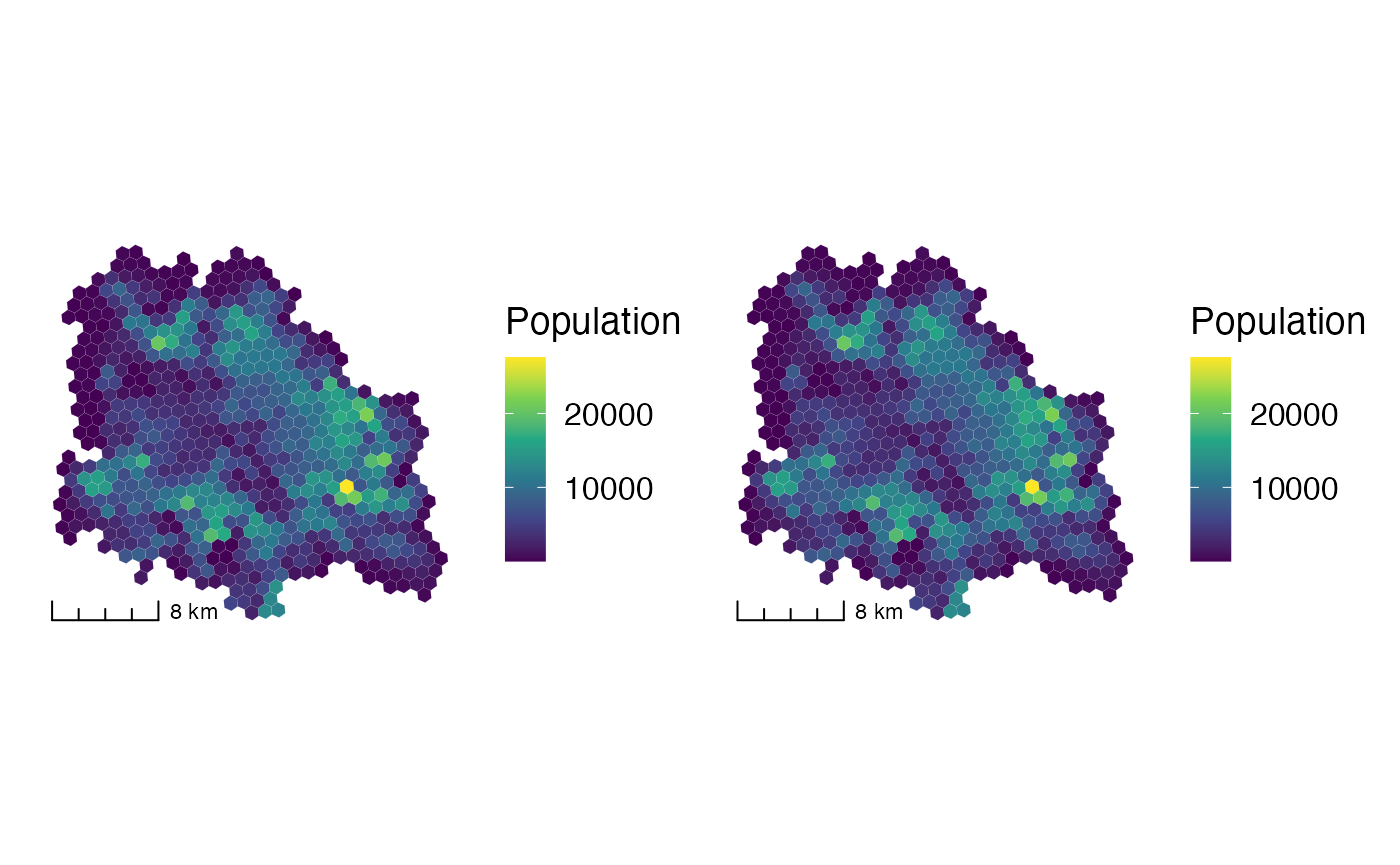
Population of the metropolitan area of Guadalajara

Extract the Population

x <- popmex::extract_pop(year = 2023,
                         cve_edo = "14",
                         locality = c("Guadalajara", "Tlaquepaque", 
                                      "Zapopan", "Tonalá"))

y <- popmex::extract_pop(year = 2022,
                         cve_edo = "14",
                         locality = c("Guadalajara", "Tlaquepaque",
                                      "Zapopan", "Tonalá"))

Visualization

Static map

a <- ggplot2::ggplot() +
    ggplot2::geom_sf(data = x,
                     ggplot2::aes(fill = population),
                     col = "white",
                     lwd = 0.01) +
    ggplot2::scale_fill_viridis_c("Population") +
    cowplot::theme_map() +
    ggspatial::annotation_scale(style = "ticks")
b <- ggplot2::ggplot() +
    ggplot2::geom_sf(data = x,
                     ggplot2::aes(fill = population),
                     col = "white",
                     lwd = 0.01) +
    ggplot2::scale_fill_viridis_c("Population") +
    cowplot::theme_map() +
    ggspatial::annotation_scale(style = "ticks")
library(patchwork)
a | b

Interactive map

a <- mapview::mapview(x,
                 zcol = "population",
                 layer.name = "Population 2023")
b <- mapview::mapview(y,
                      zcol = "population",
                      layer.name = "Population 2022")

leafsync::sync(a, b)

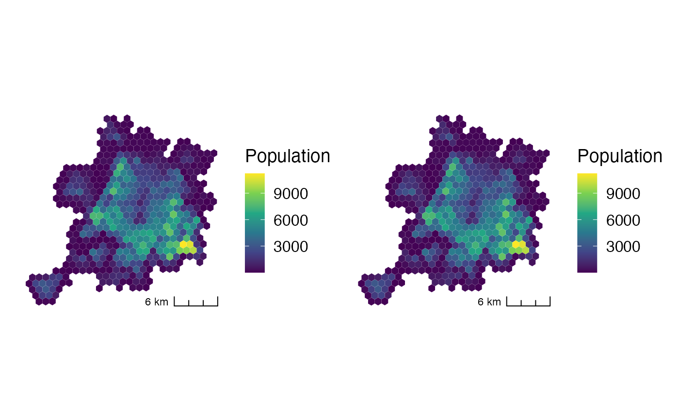
Population of the metropolitan area of Mérida

Extract the Population

x <- popmex::extract_pop(year = 2023,
                         cve_edo = "31",
                         locality = c("Merida", "Uman",
                                      "Kanasin", "Caucel",
                                      "Cholul"))

y <- popmex::extract_pop(year = 2022,
                         cve_edo = "31",
                         locality = c("Merida", "Uman",
                                      "Kanasin", "Caucel",
                                      "Cholul"))

Visualization

Static map

a <- ggplot2::ggplot() +
    ggplot2::geom_sf(data = x,
                     ggplot2::aes(fill = population),
                     col = "white",
                     lwd = 0.01) +
    ggplot2::scale_fill_viridis_c("Population") +
    cowplot::theme_map() +
    ggspatial::annotation_scale(style = "ticks", location = "br")
b <- ggplot2::ggplot() +
    ggplot2::geom_sf(data = x,
                     ggplot2::aes(fill = population),
                     col = "white",
                     lwd = 0.01) +
    ggplot2::scale_fill_viridis_c("Population") +
    cowplot::theme_map() +
    ggspatial::annotation_scale(style = "ticks", location = "br")
library(patchwork)
a | b

Interactive map

a <- mapview::mapview(x,
                 zcol = "population",
                 layer.name = "Population 2023")
b <- mapview::mapview(y,
                      zcol = "population",
                      layer.name = "Population 2022")

leafsync::sync(a, b)