Prediction of the presence of *Aedes aegypti* in the Metropolitan Area of Mexico City with LightGBM • aeaegypticdmx

Objective

Predicting the probability of the presence of Ae aegypti in Metropolitan Area of Mexico City using LightGBM

Step 1. Load the pkg

Sys.setenv("_R_CHECK_LIMIT_CORES_" = "false")
library(tidyverse) 
#> ── Attaching core tidyverse packages ──────────────────────── tidyverse 2.0.0 ──
#> ✔ dplyr     1.2.1     ✔ readr     2.2.0
#> ✔ forcats   1.0.1     ✔ stringr   1.6.0
#> ✔ ggplot2   4.0.3     ✔ tibble    3.3.1
#> ✔ lubridate 1.9.5     ✔ tidyr     1.3.2
#> ✔ purrr     1.2.2     
#> ── Conflicts ────────────────────────────────────────── tidyverse_conflicts() ──
#> ✖ dplyr::filter() masks stats::filter()
#> ✖ dplyr::lag()    masks stats::lag()
#> ℹ Use the conflicted package (<http://conflicted.r-lib.org/>) to force all conflicts to become errors
library(magrittr) 
#> 
#> Attaching package: 'magrittr'
#> 
#> The following object is masked from 'package:purrr':
#> 
#>     set_names
#> 
#> The following object is masked from 'package:tidyr':
#> 
#>     extract
library(tidymodels) # Machine Learning en R
#> ── Attaching packages ────────────────────────────────────── tidymodels 1.5.0 ──
#> ✔ broom        1.0.13     ✔ rsample      1.3.2 
#> ✔ dials        1.4.3      ✔ tailor       0.1.0 
#> ✔ infer        1.1.0      ✔ tune         2.1.0 
#> ✔ modeldata    1.5.1      ✔ workflows    1.3.0 
#> ✔ parsnip      1.6.0      ✔ workflowsets 1.1.1 
#> ✔ recipes      1.3.3      ✔ yardstick    1.4.0 
#> ── Conflicts ───────────────────────────────────────── tidymodels_conflicts() ──
#> ✖ scales::discard()     masks purrr::discard()
#> ✖ magrittr::extract()   masks tidyr::extract()
#> ✖ dplyr::filter()       masks stats::filter()
#> ✖ recipes::fixed()      masks stringr::fixed()
#> ✖ dplyr::lag()          masks stats::lag()
#> ✖ magrittr::set_names() masks purrr::set_names()
#> ✖ yardstick::spec()     masks readr::spec()
#> ✖ recipes::step()       masks stats::step()
library(skimr) 
library(bonsai)
library(themis) # Upsampling - downsampling
library(parallel)
library(doParallel)
#> Loading required package: foreach
#> 
#> Attaching package: 'foreach'
#> 
#> The following objects are masked from 'package:purrr':
#> 
#>     accumulate, when
#> 
#> Loading required package: iterators
library(sf)
#> Linking to GEOS 3.13.0, GDAL 3.8.5, PROJ 9.5.1; sf_use_s2() is TRUE

Step 2. Load the dataset and the area of interes

# Load the aedes aegypti dataset ####

data <- aeaegypticdmx::ae_aegypti_cdmx


# Step. extract the area of interes ####
aoi <-  aeaegypticdmx::aoi

Step 2.1. visualization of data and aoi

library(mapgl)
maplibre(style = carto_style("positron"),
         bounds = data) |>
    add_circle_layer(id = "Aedes aegypti",
                     source = data,
                     circle_color = match_expr(
                         column = "class",
                         values = c("presence", "pseudoabs"), # reemplaza por tus valores
                         stops = c("#E01A59", "#0F9D58")),
                     circle_stroke_color = "white", # color = "white"
                     circle_stroke_width = 0.5, # lwd = 0.5
                     circle_radius = 3) |>
    #    Capa 2 — polígono aoi (sin leyenda)
    add_fill_layer(id = "aoi",
                   source = aoi,
                   fill_color = "#ECB32D",
                   fill_opacity = 0.5, # ajusta al gusto
                   fill_outline_color = "black") |>
    add_line_layer(id           = "aoi-borde",
                   source       = aoi,      # misma fuente
                   line_color   = "black",  # color = "black"
                   line_width   = 2,        # lwd = 2
                   line_opacity = 1) |>
    add_categorical_legend(legend_title = "Aedes aegypti",
                           position = "bottom-left",
                           values = c("presence", "pseudoabs"), 
                           colors = c("#E01A59", "#0F9D58")) |>
    add_fullscreen_control(position = "top-left") |> 
    add_navigation_control()

Step 2.2. select the data of year 2024

data <- data

Step 2.3. Glimpse of your data

data |>
    dplyr::glimpse()
#> Rows: 214
#> Columns: 43
#> $ class     <fct> presence, presence, presence, presence, presence, presence, …
#> $ bio1      <dbl> 16.80292, 17.27943, 16.84335, 17.04555, 17.15956, 17.21716, …
#> $ bio10     <dbl> 18.79668, 19.25518, 18.87632, 19.03689, 19.17890, 19.21034, …
#> $ bio11     <dbl> 14.29385, 14.86375, 14.32071, 14.54662, 14.59920, 14.74367, …
#> $ bio12     <dbl> 737.8215, 615.0818, 609.4650, 659.8939, 592.1864, 589.5240, …
#> $ bio13     <dbl> 153.2636, 128.4100, 126.6036, 138.3710, 126.0558, 122.6000, …
#> $ bio14     <dbl> 7.627022, 6.519297, 7.559904, 7.000000, 6.019577, 6.056946, …
#> $ bio15     <dbl> 94.73853, 91.48577, 92.54862, 93.97945, 94.34325, 91.11935, …
#> $ bio16     <dbl> 427.1033, 349.8521, 356.8107, 385.7567, 352.1795, 336.2949, …
#> $ bio17     <dbl> 24.78072, 24.10407, 23.55990, 23.64352, 20.98487, 22.15186, …
#> $ bio18     <dbl> 211.0023, 180.9614, 185.4055, 196.4251, 183.0471, 176.3621, …
#> $ bio19     <dbl> 24.98141, 24.16955, 24.31790, 23.64352, 21.98354, 23.09491, …
#> $ bio2      <dbl> 15.96111, 16.33245, 16.02658, 15.96767, 16.28576, 16.62823, …
#> $ bio3      <dbl> 69.52179, 70.68168, 69.42849, 69.92445, 69.92628, 70.40212, …
#> $ bio4      <dbl> 182.6958, 176.5379, 184.2030, 181.9714, 186.0207, 179.9659, …
#> $ bio5      <dbl> 27.62120, 28.30707, 27.66384, 27.83565, 28.09142, 28.40000, …
#> $ bio6      <dbl> 4.662702, 5.200000, 4.580191, 5.000000, 4.801511, 4.781018, …
#> $ bio7      <dbl> 22.95850, 23.10707, 23.08365, 22.83565, 23.28991, 23.61898, …
#> $ bio8      <dbl> 18.04129, 18.41829, 18.10205, 18.29223, 18.44523, 18.41034, …
#> $ bio9      <dbl> 14.42886, 14.99826, 14.44571, 14.66875, 14.73175, 14.90272, …
#> $ dhi       <dbl> 0, 0, 0, 0, 0, 0, 0, 0, 0, 0, 0, 0, 0, 0, 0, 0, 0, 0, 0, 0, …
#> $ hfp       <dbl> 45.36700, 38.00032, 38.40737, 45.76643, 44.35675, 38.00914, …
#> $ ia        <dbl> 22.71889, 12.04736, 12.04353, 17.65742, 11.62077, 10.42579, …
#> $ ice       <dbl> 0.6822323, 0.8203631, 0.7443505, 0.7278633, 0.7636263, 0.822…
#> $ im        <dbl> 23.14940, 20.45767, 21.85011, 22.18435, 21.26418, 20.39371, …
#> $ irs       <dbl> -1.2901239, -0.9289573, -1.2362193, -1.1821170, -1.1455718, …
#> $ pop       <dbl> 9938.426, 6703.190, 16058.316, 16433.658, 8734.631, 15242.78…
#> $ indexp    <dbl> 0.018192437, 0.012953738, 0.031922441, 0.020680299, 0.028163…
#> $ suit      <dbl> 801030.1, 953743.9, 835044.3, 867783.1, 917339.9, 947860.8, …
#> $ temp      <dbl> 38.21988, 38.01561, 33.29869, 35.38102, 33.09361, 32.39949, …
#> $ built     <dbl> 0.6781858, 0.3349272, 0.7316231, 0.4295628, 0.7119719, 0.739…
#> $ tree      <dbl> 0.02521676, 0.08775567, 0.03663028, 0.09203759, 0.04561467, …
#> $ ndvi      <dbl> 0.02916859, 0.31541485, 0.22150773, 0.37087092, 0.09722266, …
#> $ psdi      <dbl> -438.6667, -120.5833, -179.5000, -218.8333, -129.4167, -109.…
#> $ prcp      <dbl> 1.616219, 1.637205, 1.625315, 1.629151, 1.620438, 1.637014, …
#> $ tmin      <dbl> 10.066904, 10.081507, 10.113507, 10.111424, 10.110767, 10.11…
#> $ tmax      <dbl> 26.46066, 26.47132, 26.45049, 26.48537, 26.45304, 26.45926, …
#> $ eddi      <dbl> 0, 0, 0, 0, 0, 0, 0, 0, 0, 0, 0, 0, 0, 0, 0, 0, 0, 0, 0, 0, …
#> $ hr        <dbl> 56.55930, 57.52564, 55.33009, 55.33009, 55.33009, 57.52564, …
#> $ elevation <dbl> 2242.407, 2241.323, 2237.703, 2239.629, 2238.717, 2234.962, …
#> $ suhi      <dbl> 0.195009023, 0.283513665, 0.115925729, 0.105637103, 0.085246…
#> $ uhi       <dbl> 21.57348, 24.23319, 19.19689, 18.88770, 18.27492, 20.45943, …
#> $ geometry  <POINT [°]> POINT (-99.16914 19.48317), POINT (-99.04132 19.36403)…

Step 2.3. EDA Univariate

# EDA Univariado ####
skimr::skim(data |> sf::st_drop_geometry())

Data summary
Name	sf::st_drop_geometry(data…
Number of rows	214
Number of columns	42
_______________________
Column type frequency:
factor	1
numeric	41
________________________
Group variables	None

Variable type: factor

skim_variable	n_missing	complete_rate	ordered	n_unique	top_counts
class	0	1	FALSE	2	pre: 121, pse: 93

Variable type: numeric

skim_variable	complete_rate	mean	sd	p0	p25	p50	p75	p100	hist
bio1	1	15.68	1.39	12.90	14.33	16.09	17.06	17.30	▂▅▂▂▇
bio10	1	17.58	1.48	14.59	16.12	18.03	19.05	19.31	▁▆▁▁▇
bio11	1	13.33	1.30	10.66	12.11	13.75	14.60	14.86	▂▅▂▂▇
bio12	1	805.70	160.89	576.59	662.41	772.51	948.64	1175.52	▇▃▃▅▁
bio13	1	168.33	33.29	121.61	137.95	162.71	198.66	245.62	▇▂▃▅▁
bio14	1	8.09	1.49	4.86	7.00	8.00	9.06	12.96	▃▇▅▂▁
bio15	1	94.62	1.93	89.89	93.00	94.68	96.31	98.49	▂▇▇▇▅
bio16	1	470.22	98.30	331.39	380.79	451.03	558.83	687.54	▇▂▂▆▁
bio17	1	28.96	5.93	19.17	24.35	26.14	34.01	46.98	▇▇▆▃▁
bio18	1	235.66	46.15	170.81	193.32	222.95	279.37	330.86	▇▃▂▆▂
bio19	1	29.20	5.94	20.00	24.48	26.19	34.64	46.98	▇▂▅▂▁
bio2	1	15.43	0.73	13.89	14.69	15.53	16.03	16.70	▂▆▅▇▃
bio3	1	70.13	1.13	67.02	69.55	70.11	70.65	72.71	▁▂▇▃▂
bio4	1	171.99	10.63	150.51	163.03	175.71	180.79	202.02	▅▃▇▅▁
bio5	1	26.13	1.89	22.62	24.23	26.86	27.90	28.40	▂▅▁▂▇
bio6	1	4.12	0.92	1.66	3.43	4.44	5.00	5.20	▁▂▃▂▇
bio7	1	22.01	1.21	19.24	20.74	22.50	22.94	24.22	▂▃▃▇▂
bio8	1	16.83	1.39	14.13	15.49	17.15	18.24	18.45	▂▅▂▂▇
bio9	1	13.39	1.34	10.66	12.11	13.89	14.67	15.01	▂▅▂▂▇
dhi	1	1.10	2.34	0.00	0.00	0.00	0.00	10.00	▇▂▁▁▁
hfp	1	40.68	3.34	30.67	38.36	40.24	43.26	48.05	▁▂▇▅▃
ia	1	16.49	3.61	8.47	13.69	15.84	19.15	25.96	▁▇▆▅▁
ice	1	0.81	0.06	0.68	0.78	0.82	0.87	0.91	▃▃▇▇▇
im	1	22.10	0.95	20.39	21.22	22.18	22.99	23.58	▆▃▆▅▇
irs	1	-1.01	0.16	-1.31	-1.09	-1.00	-0.92	-0.58	▃▇▇▃▁
pop	1	8325.17	5766.79	158.83	2604.06	8725.81	12872.92	26451.65	▇▆▆▂▁
indexp	1	0.01	0.01	0.00	0.00	0.01	0.01	0.04	▇▅▂▁▁
suit	1	630557.82	252028.84	187770.72	380877.60	677237.78	892707.94	953743.94	▃▆▁▃▇
temp	1	31.39	3.57	20.02	28.76	31.38	33.84	41.35	▁▃▇▅▁
built	1	0.64	0.17	0.03	0.64	0.72	0.74	0.77	▁▁▁▁▇
tree	1	0.06	0.08	0.02	0.03	0.04	0.05	0.62	▇▁▁▁▁
ndvi	1	0.23	0.13	0.00	0.12	0.21	0.32	0.64	▆▇▇▂▁
psdi	1	-274.20	100.44	-463.67	-352.83	-271.75	-185.83	-95.67	▃▆▃▇▃
prcp	1	1.64	0.02	1.56	1.63	1.63	1.65	1.69	▁▁▇▆▂
tmin	1	9.13	1.13	6.14	8.23	9.91	10.10	10.13	▁▂▃▂▇
tmax	1	25.80	0.80	23.66	25.19	26.39	26.48	26.56	▁▂▃▂▇
eddi	1	0.00	0.00	0.00	0.00	0.00	0.00	0.00	▁▁▇▁▁
hr	1	58.69	1.86	54.31	57.86	59.00	60.03	61.93	▃▂▇▇▆
elevation	1	2423.85	213.94	2232.05	2239.95	2268.89	2598.31	2988.24	▇▁▃▁▁
suhi	1	0.04	0.12	-0.32	-0.05	0.03	0.12	0.33	▁▅▇▇▂
uhi	1	16.66	3.96	-3.55	14.15	16.67	19.20	25.58	▁▁▃▇▂

gtExtras::gt_plt_summary(data |> sf::st_drop_geometry())

	Column	Missing	Mean	Median	SD
sf::st_drop_geometry(data)
214 rows x 42 cols
	class presence and pseudoabs	0.0%	—	—	—
	bio1	0.0%	15.7	16.1	1.4
	bio10	0.0%	17.6	18.0	1.5
	bio11	0.0%	13.3	13.8	1.3
	bio12	0.0%	805.7	772.5	160.9
	bio13	0.0%	168.3	162.7	33.3
	bio14	0.0%	8.1	8.0	1.5
	bio15	0.0%	94.6	94.7	1.9
	bio16	0.0%	470.2	451.0	98.3
	bio17	0.0%	29.0	26.1	5.9
	bio18	0.0%	235.7	223.0	46.2
	bio19	0.0%	29.2	26.2	5.9
	bio2	0.0%	15.4	15.5	0.7
	bio3	0.0%	70.1	70.1	1.1
	bio4	0.0%	172.0	175.7	10.6
	bio5	0.0%	26.1	26.9	1.9
	bio6	0.0%	4.1	4.4	0.9
	bio7	0.0%	22.0	22.5	1.2
	bio8	0.0%	16.8	17.2	1.4
	bio9	0.0%	13.4	13.9	1.3
	dhi	0.0%	1.1	0.0	2.3
	hfp	0.0%	40.7	40.2	3.3
	ia	0.0%	16.5	15.8	3.6
	ice	0.0%	0.8	0.8	0.1
	im	0.0%	22.1	22.2	1.0
	irs	0.0%	−1.0	−1.0	0.2
	pop	0.0%	8,325.2	8,725.8	5,766.8
	indexp	0.0%	0.0	0.0	0.0
	suit	0.0%	630,557.8	677,237.8	252,028.8
	temp	0.0%	31.4	31.4	3.6
	built	0.0%	0.6	0.7	0.2
	tree	0.0%	0.1	0.0	0.1
	ndvi	0.0%	0.2	0.2	0.1
	psdi	0.0%	−274.2	−271.8	100.4
	prcp	0.0%	1.6	1.6	0.0
	tmin	0.0%	9.1	9.9	1.1
	tmax	0.0%	25.8	26.4	0.8
	eddi	0.0%	0.0	0.0	0.0
	hr	0.0%	58.7	59.0	1.9
	elevation	0.0%	2,423.8	2,268.9	213.9
	suhi	0.0%	0.0	0.0	0.1
	uhi	0.0%	16.7	16.7	4.0

Step 3.4. EDA Multivariate

3.5. Weights

table

# Balanceo
data |>
    sf::st_drop_geometry() |>
    dplyr::group_by(class) |> 
    dplyr::count(name = 'frec') |>
    dplyr::ungroup() |>
    dplyr::mutate( Porc= frec/sum(frec)) |>
    gt::gt()

class	frec	Porc
presence	121	0.5654206
pseudoabs	93	0.4345794

graph

data |>
    sf::st_drop_geometry() |>
    dplyr::group_by(class) |> 
    dplyr::count(name = 'frec') |>
    dplyr::ungroup() |>
    dplyr::mutate(Porc= frec/sum(frec)) |>
    ggplot2::ggplot(ggplot2::aes(x= class, 
                                 y= Porc)) +
    ggplot2::geom_segment(ggplot2::aes(xend = class, 
                                       y = 0, 
                                       yend=Porc), 
                          color= c("#4285F4","#E01A59"), 
                          linewidth= 1) +
    ggplot2::geom_point(size=5, 
                        color= c("#4285F4","#E01A59")) +
    ggplot2::coord_flip() +
    ggplot2::scale_y_continuous(labels = scales::percent_format()) +
    ggplot2::labs(title= 'Porcentaje de Registros', 
                  y = "Porcentaje", 
                  x = "") +
    ggplot2::theme_bw()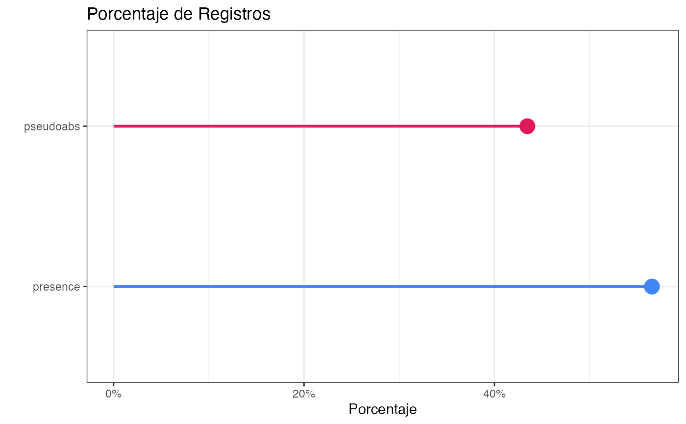

Step 4. Modeling

Step 4.1. Step Train-Test Split

initial split

# . Train-Test Split ####
set.seed(12345) # Semilla para aleatorios
split <- data |>
    rsample::initial_split(prop = 0.8, 
                           strata = class)

Train

train <- rsample::training(split)
dim(train)
#> [1] 170  43

Test

test <- rsample::testing(split)
dim(test)
#> [1] 44 43

Step 4.2. Preprocess

Importance Weights and recipe

receta <- train |>
    sf::st_drop_geometry() |>
    #dplyr::select(class, dplyr::starts_with("bio")) |>
    recipes::recipe(class ~ . ) |>## Crea la receta 
    ## Eliminar variables que no usaremos
    # step_rm() |>
    ## Crear nuevas variables (insight desde el EDA)
    #recipes::step_mutate(temperature = temperature/1000) |>
    ## Imputar los datos 
    # step_impute_mean()
    recipes::step_impute_knn(recipes::all_predictors() ) |>
    ## Estandarizacion/Normalizacion de numericas
    recipes::step_normalize(recipes::all_numeric(),
                            -recipes::all_outcomes()) |>
    ## Crear una categoría "otros" que agrupe a categorias pequeñas
    recipes::step_other(recipes::all_nominal(), 
                        -recipes::all_outcomes() , 
                        threshold = 0.07, 
                        other = "otros") |>
    ## Crear una categoría "new" para observaciones con labels "no muestreados"
    recipes::step_novel(recipes::all_nominal(), 
                        -recipes::all_outcomes(), 
                        new_level = "new") |>
    ## Crear variables indicadoras para cada categoría
    recipes::step_dummy(recipes::all_nominal(), 
                        -recipes::all_outcomes()) |># Dummy
    ## Eliminar automáticamente variables con alta correlacion 
    ## para evitar la multicolinealidad xi ~ xj
    recipes::step_corr(recipes::all_numeric(),
                       -recipes::all_outcomes(), 
                       threshold = 0.80) |>
  recipes::step_nzv(all_predictors()) |>
    # Tambien podemos eliminar variables con multicolinealidad "a mano"
    #recipes::step_rm(suhi_night, suhi_day) |>
    ## Balancear usando upsampling
    ## over_ratio implica que vamos a llevar a la clase minoritaria a 
    ## alrededor de 90% de filas que la mayoritaria
    themis::step_upsample(class, 
                          over_ratio= 0.99, 
                          skip= TRUE, 
                          seed = 345)

receta

receta |>
    recipes::prep() |>
    recipes::bake(new_data = NULL) |>
    dplyr::glimpse()
#> Rows: 191
#> Columns: 18
#> $ bio14 <dbl> -1.41039618, -0.07439577, 0.59360443, 0.59360443, -2.07839638, -…
#> $ bio15 <dbl> 0.17143475, -0.27413347, 1.00749647, 0.85319214, -1.12196597, -0…
#> $ bio3  <dbl> -0.004923246, -0.272680451, -0.355969446, -0.570423358, -2.62926…
#> $ bio4  <dbl> 0.81009973, 0.10379171, -0.52729262, -0.34790061, 1.18859553, 0.…
#> $ bio6  <dbl> 0.55922806, 0.97182143, 0.14493811, 0.70938362, -0.09399920, 0.6…
#> $ dhi   <dbl> -0.4580647, -0.4580647, -0.4580647, -0.4580647, -0.4580647, -0.4…
#> $ hfp   <dbl> -0.7904471, -0.3486069, -0.7227499, 0.3140911, 0.2635001, 1.4435…
#> $ ia    <dbl> -1.15807304, -0.37849352, 0.06234643, 0.02406640, -0.88139497, -…
#> $ im    <dbl> -1.251954353, -0.190004024, 1.267564541, 1.405952606, -1.1564958…
#> $ irs   <dbl> -0.4101527, 0.5484713, -0.3958426, -0.1301531, 2.1031932, -1.578…
#> $ pop   <dbl> -0.59650881, 0.84372138, -0.29359332, 0.84027708, 0.09175381, 1.…
#> $ built <dbl> 0.63681430, -1.75420620, 0.71389973, 0.48880545, 0.61225924, -0.…
#> $ tree  <dbl> -0.43405691, 0.05168342, -0.43416400, -0.39173236, -0.31846468, …
#> $ ndvi  <dbl> -1.04789304, 0.98163706, -0.81113063, -0.04462298, 0.68889647, 1…
#> $ prcp  <dbl> -0.51309216, -0.17542722, 0.11492133, 0.06375931, 0.12515040, -0…
#> $ hr    <dbl> -0.4458319, 0.7242051, 0.1676487, 0.1676487, 0.4619741, -1.81761…
#> $ uhi   <dbl> 0.49959916, 0.49486185, -0.11690871, 0.21909013, 0.72777063, -0.…
#> $ class <fct> presence, presence, presence, presence, presence, presence, pres…

Step 4.3. Hyperparameter Optimization and Training

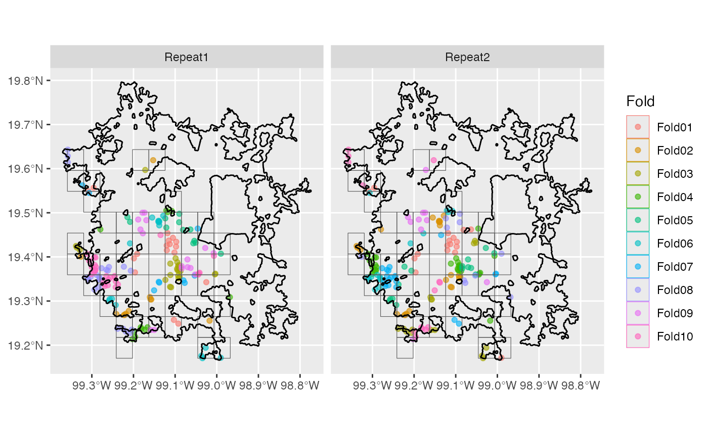
Resampling with with spatial block cross-validation

set.seed(12345)
library(tidysdm)
sp_block_cv  <- TRUE
if(sp_block_cv == TRUE){
cv <- spatialsample::spatial_block_cv(train,
                                      method = "random",
                                      repeats = 2,
                                      v = 10)
autoplot(cv) +
    ggplot2::geom_sf(data = aoi,
                     fill = NA,
                     col = "black",
                     lwd = 0.5)
} else{
cv <- rsample::vfold_cv(train |> sf::st_drop_geometry(), 
                        v = 10, 
                        repeats = 2, 
                        strata = class)
}

cv
#> #  10-fold spatial block cross-validation 
#> # A tibble: 20 × 3
#>    splits           id      id2   
#>    <list>           <chr>   <chr> 
#>  1 <split [153/17]> Repeat1 Fold01
#>  2 <split [159/11]> Repeat1 Fold02
#>  3 <split [144/26]> Repeat1 Fold03
#>  4 <split [158/12]> Repeat1 Fold04
#>  5 <split [158/12]> Repeat1 Fold05
#>  6 <split [154/16]> Repeat1 Fold06
#>  7 <split [161/9]>  Repeat1 Fold07
#>  8 <split [147/23]> Repeat1 Fold08
#>  9 <split [154/16]> Repeat1 Fold09
#> 10 <split [142/28]> Repeat1 Fold10
#> 11 <split [153/17]> Repeat2 Fold01
#> 12 <split [147/23]> Repeat2 Fold02
#> 13 <split [154/16]> Repeat2 Fold03
#> 14 <split [140/30]> Repeat2 Fold04
#> 15 <split [155/15]> Repeat2 Fold05
#> 16 <split [155/15]> Repeat2 Fold06
#> 17 <split [150/20]> Repeat2 Fold07
#> 18 <split [160/10]> Repeat2 Fold08
#> 19 <split [160/10]> Repeat2 Fold09
#> 20 <split [156/14]> Repeat2 Fold10

if(sp_block_cv == TRUE){
check_splits_balance(cv, class)
} else{
}
#> # A tibble: 20 × 4
#>    presence_assessment pseudoabs_assessment presence_analysis pseudoabs_analysis
#>                  <int>                <int>             <int>              <int>
#>  1                  81                   72                15                  2
#>  2                  91                   68                 5                  6
#>  3                  73                   71                23                  3
#>  4                  92                   66                 4                  8
#>  5                  84                   74                12                  0
#>  6                  87                   67                 9                  7
#>  7                  89                   72                 7                  2
#>  8                  94                   53                 2                 21
#>  9                  82                   72                14                  2
#> 10                  91                   51                 5                 23
#> 11                  82                   71                14                  3
#> 12                  82                   65                14                  9
#> 13                  89                   65                 7                  9
#> 14                  77                   63                19                 11
#> 15                  86                   69                10                  5
#> 16                  91                   64                 5                 10
#> 17                  91                   59                 5                 15
#> 18                  87                   73                 9                  1
#> 19                  87                   73                 9                  1
#> 20                  92                   64                 4                 10

Metrics

#. Métricas ####
library(yardstick)
library(tidysdm)
metricas <- yardstick::metric_set(roc_auc,
                                  yardstick::sens,
                                  yardstick::spec,
                                  yardstick::brier_class,
                                  yardstick::pr_auc,
                                  bal_accuracy,
                                  yardstick::pr_auc, 
                                  accuracy, 
                                  tidysdm::boyce_cont, 
                                  tidysdm::tss,
                                  tidysdm::tss_max,
                                  kap)
metricas
#> A metric set, consisting of:
#> - `roc_auc()`, a probability metric     | direction: maximize
#> - `sens()`, a class metric              | direction: maximize
#> - `spec()`, a class metric              | direction: maximize
#> - `brier_class()`, a probability metric | direction: minimize
#> - `pr_auc()`, a probability metric      | direction: maximize
#> - `bal_accuracy()`, a class metric      | direction: maximize
#> - `pr_auc()`, a probability metric      | direction: maximize
#> - `accuracy()`, a class metric          | direction: maximize
#> - `boyce_cont()`, a probability metric  | direction: maximize
#> - `tss()`, a class metric               | direction: maximize
#> - `tss_max()`, a probability metric     | direction: maximize
#> - `kap()`, a class metric               | direction: maximize

Activate Parallelization

parallel::detectCores(logical=FALSE)
#> [1] 10

cl <- parallel::makePSOCKcluster(8)
doParallel::registerDoParallel(cl)

Model specification

# =============================================================================
#  Model specification
# =============================================================================
library(bonsai)
lgbm_sp <- parsnip::boost_tree(mtry = tune::tune(), 
                               trees = tune::tune(), 
                               tree_depth = tune::tune(),
                               #min_n          = tune::tune(), 
                               #sample_size    = tune::tune(), 
                               loss_reduction = tune::tune(), 
                               learn_rate= tune::tune()) |>
    parsnip::set_engine("lightgbm") |>
    parsnip::set_mode("classification")

Workflow

# =============================================================================
# Workflow
# =============================================================================
lgbm_wflow <- workflows::workflow() |>
    workflows::add_recipe(receta) |>
    workflows::add_model(lgbm_sp) 
lgbm_wflow
#> ══ Workflow ════════════════════════════════════════════════════════════════════
#> Preprocessor: Recipe
#> Model: boost_tree()
#> 
#> ── Preprocessor ────────────────────────────────────────────────────────────────
#> 8 Recipe Steps
#> 
#> • step_impute_knn()
#> • step_normalize()
#> • step_other()
#> • step_novel()
#> • step_dummy()
#> • step_corr()
#> • step_nzv()
#> • step_upsample()
#> 
#> ── Model ───────────────────────────────────────────────────────────────────────
#> Boosted Tree Model Specification (classification)
#> 
#> Main Arguments:
#>   mtry = tune::tune()
#>   trees = tune::tune()
#>   tree_depth = tune::tune()
#>   learn_rate = tune::tune()
#>   loss_reduction = tune::tune()
#> 
#> Computational engine: lightgbm

Hyperparameter Space

Search Mesh

# =============================================================================
# Hyperparameter Space
# =============================================================================
set.seed(12345)
lgbm_grid <- lgbm_sp |>
  workflowsets::extract_parameter_set_dials() |>
  recipes::update(mtry       = dials::mtry(range= c(3, 7)),
                  trees      = dials::trees(range = c(100, 600)),
                  tree_depth = dials::tree_depth(range= c(3, 7))) |>
  dials::grid_space_filling(size = 150, 
                            type = "latin_hypercube")

lgbm_grid 
#> # A tibble: 150 × 5
#>     mtry trees tree_depth learn_rate loss_reduction
#>    <int> <int>      <int>      <dbl>          <dbl>
#>  1     4   300          5    0.0256        1.05e+ 1
#>  2     7   451          5    0.00396       2.24e- 8
#>  3     3   211          6    0.136         5.10e- 7
#>  4     7   269          7    0.215         1.51e-10
#>  5     4   530          7    0.0623        4.08e- 8
#>  6     5   136          5    0.0490        4.84e- 4
#>  7     4   374          4    0.126         6.15e+ 0
#>  8     5   168          4    0.00119       1.22e- 7
#>  9     7   561          4    0.00281       1.42e- 6
#> 10     4   334          5    0.00226       4.28e- 9
#> # ℹ 140 more rows

Training

# =============================================================================
# training
# =============================================================================
tictoc::tic()
set.seed(12345)
lgbm_tuned <- tune::tune_grid(lgbm_wflow, ## Model
                             resamples= cv, ## Crossvalidation
                             grid = lgbm_grid, ## grid search
                             metrics = metricas, ## Metrics
                             control= tune::control_grid(allow_par = T, 
                                                         verbose  = T,
                                                         save_pred = T))
tictoc::toc()
#> 175.248 sec elapsed

Sensitivity

tune::show_best(x = lgbm_tuned, metric = 'sens', n = 10)
#> # A tibble: 10 × 11
#>     mtry trees tree_depth learn_rate loss_reduction .metric .estimator  mean
#>    <int> <int>      <int>      <dbl>          <dbl> <chr>   <chr>      <dbl>
#>  1     4   383          5    0.220      2.84        sens    binary     0.971
#>  2     6   207          3    0.163     20.3         sens    binary     0.967
#>  3     6   112          7    0.00609    0.00000109  sens    binary     0.964
#>  4     3   272          4    0.277      0.00593     sens    binary     0.963
#>  5     3   233          5    0.197      0.000000962 sens    binary     0.961
#>  6     4   523          7    0.00380    0.0222      sens    binary     0.959
#>  7     3   245          3    0.00202    1.41        sens    binary     0.958
#>  8     3   284          5    0.00761    1.83        sens    binary     0.958
#>  9     6   407          5    0.0791     0.0774      sens    binary     0.958
#> 10     6   446          5    0.0664     0.00117     sens    binary     0.958
#> # ℹ 3 more variables: n <int>, std_err <dbl>, .config <chr>

Accuracy

tune::show_best(lgbm_tuned, metric = 'accuracy', n = 10)
#> # A tibble: 10 × 11
#>     mtry trees tree_depth learn_rate loss_reduction .metric  .estimator  mean
#>    <int> <int>      <int>      <dbl>          <dbl> <chr>    <chr>      <dbl>
#>  1     4   457          5    0.255         7.50e- 5 accuracy binary     0.985
#>  2     3   215          3    0.0395        1.68e- 4 accuracy binary     0.982
#>  3     3   579          4    0.108         1.05e- 7 accuracy binary     0.982
#>  4     4   560          4    0.0138        1.21e- 4 accuracy binary     0.982
#>  5     3   233          5    0.197         9.62e- 7 accuracy binary     0.980
#>  6     4   510          6    0.0108        7.35e-10 accuracy binary     0.979
#>  7     6   112          7    0.00609       1.09e- 6 accuracy binary     0.978
#>  8     3   245          3    0.00202       1.41e+ 0 accuracy binary     0.978
#>  9     3   284          5    0.00761       1.83e+ 0 accuracy binary     0.978
#> 10     3   140          6    0.0962        3.21e- 7 accuracy binary     0.978
#> # ℹ 3 more variables: n <int>, std_err <dbl>, .config <chr>

Specificity

tune::show_best(lgbm_tuned, metric = 'spec', n = 10)
#> # A tibble: 10 × 11
#>     mtry trees tree_depth learn_rate loss_reduction .metric .estimator  mean
#>    <int> <int>      <int>      <dbl>          <dbl> <chr>   <chr>      <dbl>
#>  1     3   140          6    0.0962        3.21e- 7 spec    binary         1
#>  2     3   151          5    0.0749        3.33e- 9 spec    binary         1
#>  3     3   215          3    0.0395        1.68e- 4 spec    binary         1
#>  4     3   245          3    0.00202       1.41e+ 0 spec    binary         1
#>  5     3   284          5    0.00761       1.83e+ 0 spec    binary         1
#>  6     3   318          6    0.00109       9.77e-10 spec    binary         1
#>  7     3   325          3    0.00238       1.43e- 7 spec    binary         1
#>  8     3   350          3    0.00905       6.34e- 7 spec    binary         1
#>  9     3   417          7    0.00102       6.34e- 6 spec    binary         1
#> 10     3   579          4    0.108         1.05e- 7 spec    binary         1
#> # ℹ 3 more variables: n <int>, std_err <dbl>, .config <chr>

Step 4.4. Final Model

Define the best combination of hyperparameters

In this workflow, the best combination of hyperparameters was defined using sensitivity, because the goal is to predict where dengue cases are located.

lgbm_pars_fin <- tune::select_best(lgbm_tuned, 
                                   metric = "sens")
lgbm_pars_fin
#> # A tibble: 1 × 6
#>    mtry trees tree_depth learn_rate loss_reduction .config          
#>   <int> <int>      <int>      <dbl>          <dbl> <chr>            
#> 1     4   383          5      0.220           2.84 pre0_mod039_post0

Finalize (give values to tunable parameters) the workflow

lgbm_wflow_fin <- lgbm_wflow |>
    tune::finalize_workflow(lgbm_pars_fin)
lgbm_wflow_fin
#> ══ Workflow ════════════════════════════════════════════════════════════════════
#> Preprocessor: Recipe
#> Model: boost_tree()
#> 
#> ── Preprocessor ────────────────────────────────────────────────────────────────
#> 8 Recipe Steps
#> 
#> • step_impute_knn()
#> • step_normalize()
#> • step_other()
#> • step_novel()
#> • step_dummy()
#> • step_corr()
#> • step_nzv()
#> • step_upsample()
#> 
#> ── Model ───────────────────────────────────────────────────────────────────────
#> Boosted Tree Model Specification (classification)
#> 
#> Main Arguments:
#>   mtry = 4
#>   trees = 383
#>   tree_depth = 5
#>   learn_rate = 0.219913216216053
#>   loss_reduction = 2.84263262405679
#> 
#> Computational engine: lightgbm

Step 4.5. Train the final model

lgbm_fitted <- fit(lgbm_wflow_fin, train)
lgbm_fitted
#> ══ Workflow [trained] ══════════════════════════════════════════════════════════
#> Preprocessor: Recipe
#> Model: boost_tree()
#> 
#> ── Preprocessor ────────────────────────────────────────────────────────────────
#> 8 Recipe Steps
#> 
#> • step_impute_knn()
#> • step_normalize()
#> • step_other()
#> • step_novel()
#> • step_dummy()
#> • step_corr()
#> • step_nzv()
#> • step_upsample()
#> 
#> ── Model ───────────────────────────────────────────────────────────────────────
#> LightGBM Model (17 trees)
#> Objective: binary
#> Fitted to dataset with 17 columns

Step 5. Internal Validation

Step 5.1 Metrics

denriskmxnonendemic::class_metrics(ml = lgbm_fitted,
                                   train = train,
                                   test = test,
                                   ml_title = "LightGBM Aedes aegypti (2015-2025)")

.metric	.estimator	train	test	difference
LightGBM Aedes aegypti (2015-2025)
accuracy	binary	0.98	0.98	0.01
kap	binary	0.96	0.95	0.01
sens	binary	0.98	0.96	0.02
spec	binary	0.99	1.00	-0.01
ppv	binary	0.99	1.00	-0.01
npv	binary	0.97	0.95	0.02
mcc	binary	0.96	0.95	0.01
j_index	binary	0.97	0.96	0.01
bal_accuracy	binary	0.98	0.98	0.00
detection_prevalence	binary	0.56	0.55	0.01
precision	binary	0.99	1.00	-0.01
recall	binary	0.98	0.96	0.02
f_meas	binary	0.98	0.98	0.00
auc	binary	1.00	1.00	0.00
BCI	binary	0.53	0.78	-0.25
Brier Score	binary	0.01	0.02	-0.01
AUC PR	binary	1.00	1.00	0.00
TSS	binary	0.97	0.96	0.01

Step 6. Post-analysis

lgbm_fitted |>
workflows::extract_fit_parsnip() |>
    vip::vip(geom= "col",
             num_features = 16,
              aesthetics = list(color = "white",
                                fill = "black",
                                size = 1))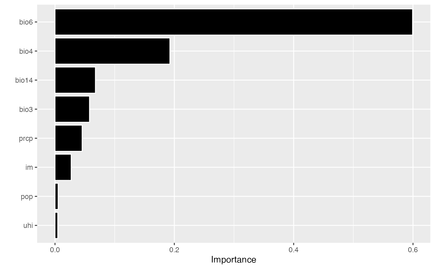

Step 7. Prediction

Step 7.1. Load the layer

library(tidyterra)
library(terra)

lyrs <- terra::rast(system.file("extdata",
                                  "raster_layers_cdmx.tif",
                                  package = "aeaegypticdmx"))  |>
    dplyr::select(-dplyr::contains("2023")) |>
    dplyr::rename(hfp = hfp2022,
                  pop = pop_2024,
                  indexp = indexp2022,
                  temp = temperature_2024,
                  built = built_2024,
                  tree = tree_2024,
                  ndvi = ndvi_2024,
                  psdi = psdi_2024,
                  prcp = prcp_2024,
                  tmin = tmin_2024,
                  tmax = tmax_2024,
                  eddi = eddi_2024,
                  hr = hr_2024,
                  suhi = suhi_2024,
                  uhi = uhi_2024)

Step 7.2. Prediction

# Make the prediction
pred <- tidysdm::predict_raster(object = lgbm_fitted, 
                                raster = lyrs,
                                type = "prob")
# Extract the predictions from the area of interest
pred <- terra::crop(x = pred,
                    y = aoi,
                    mask = TRUE)

Step 7.3. Visualization

library(mapgl)
library(terra)
maplibre_view(pred[[1]], 
              palette = viridis::turbo) |>
    add_continuous_legend(legend_title = "Probabilidad",
                          position = "bottom-left",
                          values = c(0, 0.25, 0.50, 0.75, 1),
                          colors = viridis::turbo(n = 10)) |>
  add_fullscreen_control(position = "top-left") |> 
  add_navigation_control()

Step 8. Stop Cluster

parallel::stopCluster(cl)

Step 9. Session Info

sessioninfo::session_info()
#> ─ Session info ───────────────────────────────────────────────────────────────
#>  setting  value
#>  version  R version 4.6.0 (2026-04-24)
#>  os       macOS Tahoe 26.3.1
#>  system   aarch64, darwin23
#>  ui       X11
#>  language en
#>  collate  en_US.UTF-8
#>  ctype    en_US.UTF-8
#>  tz       America/Mexico_City
#>  date     2026-06-15
#>  pandoc   3.8.3 @ /Applications/RStudio.app/Contents/Resources/app/quarto/bin/tools/aarch64/ (via rmarkdown)
#>  quarto   1.8.27 @ /usr/local/bin/quarto
#> 
#> ─ Packages ───────────────────────────────────────────────────────────────────
#>  package             * version    date (UTC) lib source
#>  aeaegypticdmx         0.1.0      2026-06-15 [1] local
#>  backports             1.5.1      2026-04-03 [2] CRAN (R 4.6.0)
#>  base64enc             0.1-6      2026-02-02 [2] CRAN (R 4.6.0)
#>  bonsai              * 0.4.1      2026-05-21 [2] CRAN (R 4.6.0)
#>  broom               * 1.0.13     2026-05-14 [2] CRAN (R 4.6.0)
#>  bslib                 0.11.0     2026-05-16 [2] CRAN (R 4.6.0)
#>  cachem                1.1.0      2024-05-16 [2] CRAN (R 4.6.0)
#>  class                 7.3-23     2025-01-01 [2] CRAN (R 4.6.0)
#>  classInt              0.4-11     2025-01-08 [2] CRAN (R 4.6.0)
#>  cli                   3.6.6      2026-04-09 [2] CRAN (R 4.6.0)
#>  codetools             0.2-20     2024-03-31 [2] CRAN (R 4.6.0)
#>  DALEX                 2.5.3      2025-10-16 [2] CRAN (R 4.6.0)
#>  data.table            1.18.4     2026-05-06 [2] CRAN (R 4.6.0)
#>  DBI                   1.3.0      2026-02-25 [2] CRAN (R 4.6.0)
#>  denriskmxnonendemic   0.1.0      2026-06-05 [2] Github (fdzul/denriskmxnonendemic@4d0bbb5)
#>  desc                  1.4.3      2023-12-10 [2] CRAN (R 4.6.0)
#>  dials               * 1.4.3      2026-04-11 [2] CRAN (R 4.6.0)
#>  DiceDesign            1.10       2023-12-07 [2] CRAN (R 4.6.0)
#>  digest                0.6.39     2025-11-19 [2] CRAN (R 4.6.0)
#>  doParallel          * 1.0.17     2022-02-07 [2] CRAN (R 4.6.0)
#>  dplyr               * 1.2.1      2026-04-03 [2] CRAN (R 4.6.0)
#>  e1071                 1.7-17     2025-12-18 [2] CRAN (R 4.6.0)
#>  evaluate              1.0.5      2025-08-27 [2] CRAN (R 4.6.0)
#>  farver                2.1.2      2024-05-13 [2] CRAN (R 4.6.0)
#>  fastmap               1.2.0      2024-05-15 [2] CRAN (R 4.6.0)
#>  fontawesome           0.5.3      2024-11-16 [2] CRAN (R 4.6.0)
#>  forcats             * 1.0.1      2025-09-25 [2] CRAN (R 4.6.0)
#>  foreach             * 1.5.2      2022-02-02 [2] CRAN (R 4.6.0)
#>  fs                    2.1.0      2026-04-18 [2] CRAN (R 4.6.0)
#>  furrr                 0.4.0      2026-03-31 [2] CRAN (R 4.6.0)
#>  future                1.70.0     2026-03-14 [2] CRAN (R 4.6.0)
#>  future.apply          1.20.2     2026-02-20 [2] CRAN (R 4.6.0)
#>  generics              0.1.4      2025-05-09 [2] CRAN (R 4.6.0)
#>  geojsonsf             2.0.5      2025-11-26 [2] CRAN (R 4.6.0)
#>  ggplot2             * 4.0.3      2026-04-22 [2] CRAN (R 4.6.0)
#>  globals               0.19.1     2026-03-13 [2] CRAN (R 4.6.0)
#>  glue                  1.8.1      2026-04-17 [2] CRAN (R 4.6.0)
#>  gower                 1.0.2      2024-12-17 [2] CRAN (R 4.6.0)
#>  gridExtra             2.3        2017-09-09 [2] CRAN (R 4.6.0)
#>  gt                    1.3.0      2026-01-22 [2] CRAN (R 4.6.0)
#>  gtable                0.3.6      2024-10-25 [2] CRAN (R 4.6.0)
#>  gtExtras              0.6.2      2026-01-17 [2] CRAN (R 4.6.0)
#>  hardhat               1.4.3      2026-04-04 [2] CRAN (R 4.6.0)
#>  hms                   1.1.4      2025-10-17 [2] CRAN (R 4.6.0)
#>  htmltools             0.5.9      2025-12-04 [2] CRAN (R 4.6.0)
#>  htmlwidgets           1.6.4      2023-12-06 [2] CRAN (R 4.6.0)
#>  infer               * 1.1.0      2025-12-18 [2] CRAN (R 4.6.0)
#>  ipred                 0.9-15     2024-07-18 [2] CRAN (R 4.6.0)
#>  iterators           * 1.0.14     2022-02-05 [2] CRAN (R 4.6.0)
#>  jquerylib             0.1.4      2021-04-26 [2] CRAN (R 4.6.0)
#>  jsonlite              2.0.0      2025-03-27 [2] CRAN (R 4.6.0)
#>  KernSmooth            2.23-26    2025-01-01 [2] CRAN (R 4.6.0)
#>  knitr                 1.51       2025-12-20 [2] CRAN (R 4.6.0)
#>  labeling              0.4.3      2023-08-29 [2] CRAN (R 4.6.0)
#>  lattice               0.22-9     2026-02-09 [2] CRAN (R 4.6.0)
#>  lava                  1.9.1      2026-05-14 [2] CRAN (R 4.6.0)
#>  lifecycle             1.0.5      2026-01-08 [2] CRAN (R 4.6.0)
#>  lightgbm              4.6.0      2025-02-13 [2] CRAN (R 4.6.0)
#>  listenv               0.10.1     2026-03-10 [2] CRAN (R 4.6.0)
#>  lubridate           * 1.9.5      2026-02-04 [2] CRAN (R 4.6.0)
#>  magrittr            * 2.0.5      2026-04-04 [2] CRAN (R 4.6.0)
#>  mapgl               * 0.4.6      2026-04-14 [2] CRAN (R 4.6.0)
#>  MASS                  7.3-65     2025-02-28 [2] CRAN (R 4.6.0)
#>  Matrix                1.7-5      2026-03-21 [2] CRAN (R 4.6.0)
#>  Metrics               0.1.4      2018-07-09 [2] CRAN (R 4.6.0)
#>  mirai                 2.7.1      2026-06-01 [2] CRAN (R 4.6.0)
#>  modeldata           * 1.5.1      2025-08-22 [2] CRAN (R 4.6.0)
#>  nanonext              1.9.1      2026-06-01 [2] CRAN (R 4.6.0)
#>  nnet                  7.3-20     2025-01-01 [2] CRAN (R 4.6.0)
#>  otel                  0.2.0      2025-08-29 [2] CRAN (R 4.6.0)
#>  paletteer             1.7.0      2026-01-08 [2] CRAN (R 4.6.0)
#>  parallelly            1.47.0     2026-04-17 [2] CRAN (R 4.6.0)
#>  parsnip             * 1.6.0      2026-05-14 [2] CRAN (R 4.6.0)
#>  pillar                1.11.1     2025-09-17 [2] CRAN (R 4.6.0)
#>  pkgconfig             2.0.3      2019-09-22 [2] CRAN (R 4.6.0)
#>  pkgdown               2.2.0      2025-11-06 [2] CRAN (R 4.6.0)
#>  prodlim               2026.03.11 2026-03-11 [2] CRAN (R 4.6.0)
#>  proxy                 0.4-29     2025-12-29 [2] CRAN (R 4.6.0)
#>  purrr               * 1.2.2      2026-04-10 [2] CRAN (R 4.6.0)
#>  R6                    2.6.1      2025-02-15 [2] CRAN (R 4.6.0)
#>  ragg                  1.5.2      2026-03-23 [2] CRAN (R 4.6.0)
#>  RColorBrewer          1.1-3      2022-04-03 [2] CRAN (R 4.6.0)
#>  Rcpp                  1.1.1-1.1  2026-04-24 [2] CRAN (R 4.6.0)
#>  readr               * 2.2.0      2026-02-19 [2] CRAN (R 4.6.0)
#>  recipes             * 1.3.3      2026-05-30 [2] CRAN (R 4.6.0)
#>  rematch2              2.1.2      2020-05-01 [2] CRAN (R 4.6.0)
#>  repr                  1.1.7      2024-03-22 [2] CRAN (R 4.6.0)
#>  rlang                 1.2.0      2026-04-06 [2] CRAN (R 4.6.0)
#>  rmarkdown             2.31       2026-03-26 [2] CRAN (R 4.6.0)
#>  ROSE                  0.0-4      2021-06-14 [2] CRAN (R 4.6.0)
#>  rpart                 4.1.27     2026-03-27 [2] CRAN (R 4.6.0)
#>  rsample             * 1.3.2      2026-01-30 [2] CRAN (R 4.6.0)
#>  rstudioapi            0.18.0     2026-01-16 [2] CRAN (R 4.6.0)
#>  s2                    1.1.11     2026-06-01 [2] CRAN (R 4.6.0)
#>  S7                    0.2.2      2026-04-22 [2] CRAN (R 4.6.0)
#>  sass                  0.4.10     2025-04-11 [2] CRAN (R 4.6.0)
#>  scales              * 1.4.0      2025-04-24 [2] CRAN (R 4.6.0)
#>  sessioninfo           1.2.4      2026-06-04 [2] CRAN (R 4.6.0)
#>  sf                  * 1.1-1      2026-05-06 [2] CRAN (R 4.6.0)
#>  skimr               * 2.2.2      2026-01-10 [2] CRAN (R 4.6.0)
#>  sparsevctrs           0.3.6      2026-01-27 [2] CRAN (R 4.6.0)
#>  spatialsample       * 0.6.1      2025-12-02 [2] CRAN (R 4.6.0)
#>  stringi               1.8.7      2025-03-27 [2] CRAN (R 4.6.0)
#>  stringr             * 1.6.0      2025-11-04 [2] CRAN (R 4.6.0)
#>  survival              3.8-6      2026-01-16 [2] CRAN (R 4.6.0)
#>  svglite               2.2.2      2025-10-21 [2] CRAN (R 4.6.0)
#>  systemfonts           1.3.2      2026-03-05 [2] CRAN (R 4.6.0)
#>  tailor              * 0.1.0      2025-08-25 [2] CRAN (R 4.6.0)
#>  terra               * 1.9-27     2026-05-10 [2] CRAN (R 4.6.0)
#>  textshaping           1.0.5      2026-03-06 [2] CRAN (R 4.6.0)
#>  themis              * 1.0.3      2025-01-23 [2] CRAN (R 4.6.0)
#>  tibble              * 3.3.1      2026-01-11 [2] CRAN (R 4.6.0)
#>  tictoc                1.2.1      2024-03-18 [2] CRAN (R 4.6.0)
#>  tidymodels          * 1.5.0      2026-04-23 [2] CRAN (R 4.6.0)
#>  tidyr               * 1.3.2      2025-12-19 [2] CRAN (R 4.6.0)
#>  tidysdm             * 1.0.4      2025-12-13 [2] CRAN (R 4.6.0)
#>  tidyselect            1.2.1      2024-03-11 [2] CRAN (R 4.6.0)
#>  tidyterra           * 1.1.0      2026-03-11 [2] CRAN (R 4.6.0)
#>  tidyverse           * 2.0.0      2023-02-22 [2] CRAN (R 4.6.0)
#>  timechange            0.4.0      2026-01-29 [2] CRAN (R 4.6.0)
#>  timeDate              4052.112   2026-01-28 [2] CRAN (R 4.6.0)
#>  tune                * 2.1.0      2026-04-17 [2] CRAN (R 4.6.0)
#>  tzdb                  0.5.0      2025-03-15 [2] CRAN (R 4.6.0)
#>  units                 1.0-1      2026-03-11 [2] CRAN (R 4.6.0)
#>  utf8                  1.2.6      2025-06-08 [2] CRAN (R 4.6.0)
#>  vctrs                 0.7.3      2026-04-11 [2] CRAN (R 4.6.0)
#>  vip                   0.4.6      2026-04-23 [2] CRAN (R 4.6.0)
#>  viridis               0.6.5      2024-01-29 [2] CRAN (R 4.6.0)
#>  viridisLite           0.4.3      2026-02-04 [2] CRAN (R 4.6.0)
#>  withr                 3.0.2      2024-10-28 [2] CRAN (R 4.6.0)
#>  wk                    0.9.5      2025-12-18 [2] CRAN (R 4.6.0)
#>  workflows           * 1.3.0      2025-08-27 [2] CRAN (R 4.6.0)
#>  workflowsets        * 1.1.1      2025-05-27 [2] CRAN (R 4.6.0)
#>  xfun                  0.58       2026-06-01 [2] CRAN (R 4.6.0)
#>  xml2                  1.5.2      2026-01-17 [2] CRAN (R 4.6.0)
#>  yaml                  2.3.12     2025-12-10 [2] CRAN (R 4.6.0)
#>  yardstick           * 1.4.0      2026-04-07 [2] CRAN (R 4.6.0)
#> 
#>  [1] /private/var/folders/jn/bfwcn2ls0sdclpxn9r_gkbz00000gn/T/RtmpMHLDU7/temp_libpath1a3314fa6cf7
#>  [2] /Library/Frameworks/R.framework/Versions/4.6/Resources/library
#>  * ── Packages attached to the search path.
#> 
#> ──────────────────────────────────────────────────────────────────────────────

Prediction of the presence of Aedes aegypti in the Metropolitan Area of Mexico City with LightGBM

Objective

Step 1. Load the pkg

Step 2. Load the dataset and the area of interes

Step 2.1. visualization of data and aoi

Step 2.2. select the data of year 2024

Step 2.3. Glimpse of your data

Step 2.3. EDA Univariate

Step 3.4. EDA Multivariate

3.5. Weights

table

graph

Step 4. Modeling

Step 4.1. Step Train-Test Split

initial split

Train

Test

Step 4.2. Preprocess

Importance Weights and recipe

Step 4.3. Hyperparameter Optimization and Training

Resampling with with spatial block cross-validation

Metrics

Activate Parallelization

Model specification

Workflow

Hyperparameter Space

Search Mesh

Training

Step 4.4. Final Model

Define the best combination of hyperparameters

In this workflow, the best combination of hyperparameters was defined using sensitivity, because the goal is to predict where dengue cases are located.

Finalize (give values to tunable parameters) the workflow

Step 4.5. Train the final model

Step 5. Internal Validation

Step 5.1 Metrics

Step 6. Post-analysis

Step 7. Prediction

Step 7.1. Load the layer

Step 7.2. Prediction

Step 7.3. Visualization

Step 8. Stop Cluster

Step 9. Session Info